Orbital Mechanics

Newton's Law of Gravity

The N-body Problem

We are interested in the motion of n particles or masses interacting with each other via
mutual gravitation. We will denote the mass of each particle as $m_{i}$ and the position and
velocity of each particle as $r_{i}$ and $v_{i}$ respectively1.
We can denote the distance between two bodies i and j as

r_{i j} := | | r_{i} - r_{j} | | = \sqrt{(r_{i} - r_{j})^{⊤} (r_{i} - r_{j})} .

Theorem

Newton's Law of Universal Gravitation for N bodies For a system of N particles each with mass $m_{i}$ and position $r_{i}$ , the total force experienced by particle i is:

f_{i} = \sum_{j = 1, i \neq j}^{N} G \frac{m_{i} m_{j} (r_{j} - r_{i})}{r_{i j}^{3}}

the force on body i is directed raidially towards particle j in the direction of the unit vector $(r_{j} - r_{i}) / r_{i j}$

Fact

Equations of motion for N bodies For an N-body system, the equations of motion are:

\frac{d^{2} r_{i}}{d t^{2}} = \sum_{j = 1, i e q j}^{N} G \frac{m_{j} (r_{j} - r_{i})}{r_{i j}^{3}}

2 body problem

For a system of two bodies, our equations of motion are:

m_{1} \frac{d^{2} r_{1}}{d t^{2}} = G \frac{m_{1} m_{2} (r_{2} - r_{1})}{r_{12}^{3}}

m_{2} \frac{d^{2} r_{2}}{d t^{2}} = G \frac{m_{1} m_{2} (r_{1} - r_{2})}{r_{21}^{3}} .

However, we generally are more interested in the relative motion of the two bodies. We can therefore define

r := r_{2} - r_{1}

v := v_{2} - v_{1}

r := | | r | | = | | r_{2} - r_{1} | |

μ := G (m_{1} + m_{2})

so taking the difference of the above 2 equations we get

\frac{d^{2} r}{d t^{2}} + μ \frac{r}{r^{3}} = 0.

which is what we call the fundamental ODE of the 2 body problem

however notice that this implies

\frac{d}{d t} (r \times v) = \frac{d}{d t} r \times v + r \times \frac{d}{d t} v = v \times v + r \times (- \frac{μ}{r^{3}} r) = 0,

so we conclude immediately that

r \times v = h = constant

we denote $h$ to be the (specific) angular momentum vector

Corollary

we may also derive the eccentricity vector $e$ from

\frac{d}{d t} [v \times h - μ \frac{r}{r}] = 0

in which we obtain

v \times h - μ \frac{r}{r} = μ e = constant

its magnitude $e$ is known as the eccentricity of the orbit

Proof.
Step 1: Compute the Time Derivative

Consider the expression $v \times h - \frac{μ}{r} r$ and take its time derivative:

\frac{d}{d t} (v \times h - \frac{μ}{r} r) = \frac{d}{d t} (v \times h) + \frac{d}{d t} (- \frac{μ}{r} r)

Compute each term separately.

Step 2: Derivative of $v \times h$

Using the product rule for cross products:

\frac{d}{d t} (v \times h) = \frac{d v}{d t} \times h + v \times \frac{d h}{d t}

Since $h = r \times v$ is constant (from the first verification), its derivative is:

\frac{d h}{d t} = 0

Thus:

\frac{d}{d t} (v \times h) = \frac{d v}{d t} \times h + v \times 0 = \frac{d v}{d t} \times h

Substitute the acceleration:

\frac{d v}{d t} = - \frac{μ}{r^{3}} r

So:

\frac{d}{d t} (v \times h) = (- \frac{μ}{r^{3}} r) \times h = - \frac{μ}{r^{3}} (r \times h)

Since $h = r \times v$ , substitute this in:

r \times h = r \times (r \times v)

Use the vector triple product identity $A \times (B \times C) = B (A \cdot C) - C (A \cdot B)$ , with $A = r$ , $B = r$ , $C = v$ :

r \times (r \times v) = r (r \cdot v) - v (r \cdot r)

Since $r \cdot r = r^{2}$ :

r \times h = r (r \cdot v) - v r^{2}

Now:

- \frac{μ}{r^{3}} (r \times h) = - \frac{μ}{r^{3}} [r (r \cdot v) - v r^{2}]

Distribute:

= - \frac{μ}{r^{3}} r (r \cdot v) + \frac{μ}{r^{3}} v r^{2} = - μ \frac{r \cdot v}{r^{3}} r + μ \frac{r^{2}}{r^{3}} v = - μ \frac{r \cdot v}{r^{3}} r + μ \frac{1}{r} v

So:

\frac{d}{d t} (v \times h) = - μ \frac{r \cdot v}{r^{3}} r + μ \frac{1}{r} v

Step 3: Derivative of $- \frac{μ}{r} r$

Rewrite $- \frac{μ}{r} r = - μ \cdot \frac{r}{r}$ , where $μ$ is constant:

\frac{d}{d t} (- \frac{μ}{r} r) = - μ \frac{d}{d t} (\frac{r}{r})

Use the product rule for $\frac{r}{r} = r \cdot r^{- 1}$ :

\frac{d}{d t} (\frac{r}{r}) = \frac{d r}{d t} \cdot r^{- 1} + r \cdot \frac{d}{d t} (r^{- 1})

Since $\frac{d r}{d t} = v$ and $r^{- 1} = \frac{1}{r}$ :

\frac{d}{d t} (r^{- 1}) = \frac{d}{d t} (\frac{1}{r}) = - \frac{1}{r^{2}} \frac{d r}{d t}

Compute $\frac{d r}{d t}$ :

r = | r | = (x^{2} + y^{2} + z^{2})^{1 / 2}, \frac{d r}{d t} = \frac{r \cdot \frac{d r}{d t}}{r} = \frac{r \cdot v}{r}

So:

\frac{d}{d t} (r^{- 1}) = - \frac{1}{r^{2}} \cdot \frac{r \cdot v}{r} = - \frac{r \cdot v}{r^{3}}

Thus:

\frac{d}{d t} (\frac{r}{r}) = v \cdot \frac{1}{r} + r \cdot (- \frac{r \cdot v}{r^{3}}) = \frac{v}{r} - \frac{r \cdot v}{r^{3}} r

So:

\frac{d}{d t} (- \frac{μ}{r} r) = - μ (\frac{v}{r} - \frac{r \cdot v}{r^{3}} r) = - μ \frac{v}{r} + μ \frac{r \cdot v}{r^{3}} r

Alternatively, use the product rule directly:

\frac{d}{d t} (\frac{r}{r}) = \frac{d}{d t} (r^{- 1}) r + r^{- 1} \frac{d r}{d t} = (- \frac{r \cdot v}{r^{3}}) r + \frac{v}{r}

\frac{d}{d t} (- \frac{μ}{r} r) = - μ (- \frac{r \cdot v}{r^{3}} r + \frac{v}{r}) = μ \frac{r \cdot v}{r^{3}} r - μ \frac{v}{r}

Step 4: Combine the Results

Now, sum the derivatives:

\frac{d}{d t} (v \times h - \frac{μ}{r} r) = (- μ \frac{r \cdot v}{r^{3}} r + μ \frac{1}{r} v) + (μ \frac{r \cdot v}{r^{3}} r - μ \frac{1}{r} v)

Combine like terms:

$r$ terms: $- μ \frac{r \cdot v}{r^{3}} r + μ \frac{r \cdot v}{r^{3}} r = 0$
$v$ terms: $μ \frac{1}{r} v - μ \frac{1}{r} v = 0$

\frac{d}{d t} (v \times h - \frac{μ}{r} r) = 0

$◻$

Theorem

This equation can be then rearranged to give the orbital equation by taking its dot product with the position vector $r$

r = \frac{h^{2}}{μ} \frac{1}{1 + e \cos θ} or r = \frac{p}{1 + e \cos θ}

where $p$ is the parameter of the orbit defined by $p = \frac{h^{2}}{μ}$

Proof:

Step 3: Take the Dot Product with the Position Vector r
Following the image's hint, we take the dot product of the LRL vector A with the position vector r:

r \cdot A = r \cdot (v \times h - μ \frac{r}{r})

Using the distributive property of the dot product, this splits into two terms:

r \cdot A = r \cdot (v \times h) - r \cdot (μ \frac{r}{r})

Step 4: Compute Each Term
First Term: $r \cdot (v \times h)$
Use the scalar triple product identity:
$r \cdot (v \times h) = (r \times v) \cdot h$
Since $h = r \times v$ , substitute:
$(r \times v) \cdot h = h \cdot h$
The dot product of a vector with itself is the square of its magnitude:
$h \cdot h = h^{2}$
So:
$r \cdot (v \times h) = h^{2}$
Second Term: $r \cdot (μ_{r}^{r})$
Compute:
$r \cdot (μ_{r}^{r}) = μ \frac{r \cdot r}{r}$
Since $r \cdot r = r^{2}$ :
$μ \frac{r \cdot r}{r} = μ \frac{r^{2}}{r} = μ r$
Combine:
$r \cdot A = h^{2} - μ r$

Step 5: Express the Dot Product Geometrically
Since A is a constant vector, the dot product $r \cdot A$ can also be written as:

r \cdot A = r A \cos θ

where:

A = | A |

is the magnitude of the LRL vector.

$θ$ is the angle between r and A. In orbital mechanics, with the periapsis at

θ = 0

, A aligns with the periapsis direction, so $θ$ is the true anomaly.
Thus:

r A \cos θ = h^{2} - μ r

Step 6: Solve for $r$
Rearrange the equation to isolate terms involving $r$ :

r A \cos θ + μ r = h^{2}

Factor out $r$ :

r (A \cos θ + μ) = h^{2}

Solve for $r$ :

r = \frac{h^{2}}{A \cos θ + μ}

Step 7: Convert to Standard Orbital Equation Form
Rewrite the expression to resemble the orbital equation:

r = \frac{h^{2}}{μ + A \cos θ} = \frac{\frac{h^{2}}{μ}}{1 + \frac{A}{μ} \cos θ}

Compare this to the standard form:

r = \frac{p}{1 + e \cos θ}

• The semi-latus rectum is:

p = \frac{h^{2}}{μ}

• The eccentricity is:

e = \frac{A}{μ}

Since $A = μ e$ (from the properties of the LRL vector), this confirms:

\frac{A}{μ} = \frac{μ e}{μ} = e

Thus:

r = \frac{h^{2} / μ}{1 + e \cos θ} = \frac{p}{1 + e \cos θ}

Finally we define

Definition

The total mechanical energy per unit mass of the system

E = \frac{1}{2} v^{2} - \frac{μ}{r} = constant

To sum up what we have so far we essentially have shown

Theorem

Kepler's First Law
Each of the planets orbits the sun in an ellipse with the sun at once focus

this is a restatement of the equation of orbit just above

Theorem

Kepler's Second Law
A line joining a planet to the sun sweeps out equal areas in equal times

This law can be verified by writing the position and velocity vectors in cylindrical coordinates

r = r {\hat{r}}_{r}

v = \frac{d r}{d t} {\hat{r}}_{r} + r \frac{d θ}{d t} {\hat{r}}_{θ}

so that

r \times v = r^{2} \frac{d θ}{d t} {\hat{r}}_{z} = h .

The angular momentum vector h is constant, and its magnitude

h = r^{2} \frac{d θ}{d t} = 2 \frac{d A}{d t}

is proportional to the rate at which the radius vector sweeps out area.

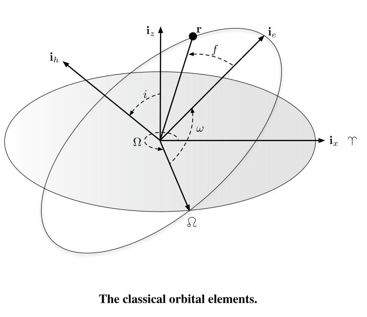
5. Coordinate Systems and Orbital Elements

Attachments/Pasted image 20250626234303.png

State Vector and Orbital Elements

ECI frame(earth centered intertial)

$i_{x}$ unit vector in the direction of the mean vernal equinox on 1 January 2000 at 12:00:00.00. (Sometimes denoted as $Υ$ in reference to the constellation Aries).
$i_{z}$ unit vector in the direction of the Earth's mean rotation axis on 1 January 2000 at 12:00:00.00.
$i_{y}$ completes the set, i.e. $i_{y} = i_{z} \times i_{x}$ .

ECEF(earth centered earth fixed)

$i_{X}$ vector in the direction of the intersection of the Greenwich meridian with the equatorial plane.
$i_{Z}$ vector in the direction of the Earth's rotation axis, coincides with $i_{z}$
$i_{Y}$ completes the set, i.e. $i_{y} = i_{z} \times i_{x}$ .

Remark

therefore the vectors $i_{X}, i_{Y}$ are attached to the earth surface and rotate once a day. The angle between $i_{X}$ and $i_{x}$ is the greenwhich mean sideral time $θ_{GMST}$ which can be measured in hours or degrees

just consider that

1 h = 15^{\circ} and θ_{GMST} = ω_{\oplus} (t - t_{0})

and obviously we can relate ECI coordinates with ECEF coordinates through a rotation matrix in the x,y plane like so

{\begin{matrix} X \\ Y \\ Z \end{matrix}} = R_{3} [θ_{GMST}] = [\begin{matrix} \cos θ_{GMST} & \sin θ_{GMST} & 0 \\ - \sin θ_{GMST} & \cos θ_{GMST} & 0 \\ 0 & 0 & 1 \end{matrix}] {\begin{matrix} x \\ y \\ z \end{matrix}} .

which is just anticlockwise by $θ_{GMST}$ from ECI. Makes sense

Perifocal Frame

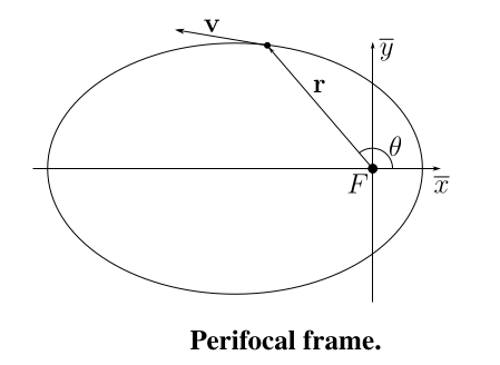
Attachments/Pasted image 20250627013155.png

$i_{e} = e / e$ vector directed along the eccentricity vector, pointing towards periapsis.
$i_{p}$ completes the set, $i_{p} = i_{h} \times i_{e}$ .
$i_{h} = h / h$ vector directed along the angular momentum vector, out of the orbital plane.

The plane $(\hat{x}, \hat{y})$ is the orbital plane. In perifocal coordinates we have

r = \overset{―}{x} i_{e} + \overset{―}{y} i_{p}

v = \overset{―}{x} i_{e} + \overset{―}{y} i_{p} .

note that

\overset{―}{x} = r \cos θ, \dot{\overset{―}{x}} = \dot{r} \cos θ - r \dot{θ} \sin θ

\overset{―}{y} = r \sin θ, \dot{\overset{―}{y}} = \dot{r} \sin θ + r \dot{θ} \cos θ .

Proposition

we have that

\dot{r} = \frac{μ}{h} e \sin θ

given that $\dot{θ} = h / r^{2}$ (by kepler's second law above)

Rewrite the orbit equation as a product:

r (1 + e \cos θ) = \frac{h^{2}}{μ}

Since the right-hand side is constant, differentiate both sides:

\frac{d}{d t} [r (1 + e \cos θ)] = 0

Apply the product rule:

\dot{r} (1 + e \cos θ) + r \cdot \frac{d}{d t} (1 + e \cos θ) = 0

From Step 4:

\frac{d}{d t} (1 + e \cos θ) = - e \sin θ \dot{θ}

So:

\dot{r} (1 + e \cos θ) + r (- e \sin θ \dot{θ}) = 0

\dot{r} (1 + e \cos θ) = r e \sin θ \dot{θ}

\dot{r} = \frac{r e \sin θ \dot{θ}}{1 + e \cos θ}

Substitute $\dot{θ} = \frac{h}{r^{2}}$ :

\dot{r} = \frac{r e \sin θ \cdot \frac{h}{r^{2}}}{1 + e \cos θ} = \frac{e \sin θ \cdot h / r}{1 + e \cos θ}

Now, use $1 + e \cos θ = \frac{h^{2} / μ}{r}$ :

\dot{r} = \frac{\frac{e \sin θ h}{r}}{\frac{h^{2} / μ}{r}} = \frac{e \sin θ h}{r} \cdot \frac{r μ}{h^{2}} = \frac{e \sin θ h μ}{h^{2}} = \frac{μ e \sin θ}{h}

so essentially it is now clear to see we can write

Fact

position and velocity and perifocal frame is

r = \frac{h^{2}}{μ} \frac{1}{1 + e \cos θ} (\cos θ i_{e} + \sin θ i_{p})

v = \frac{μ}{h} [- \sin θ i_{e} + (e + \cos θ) i_{p}] .

State Vector and Orbital Elements

Attachments/Pasted image 20250627014757.png
recall: $i_{p} = i_{h} \times i_{e}$

Definition

Consider the 6 classical orbital elements

$a$ the semimajor axis

$e$ the eccentricity
$i$ the inclination
$Ω$ the right ascension of the ascending node (RAAN)
$ω$ the argument of periapsis
$θ$ the true anomaly

To obtainj the position and velocity in the inertial frame, $r_{I}, v_{I}$ we need to rotate the perifocal frame into the inertial frame. We are not chaning $r$ we merely rotating the coordinate axes! In particular we have

\begin{aligned} r_{I} & = A r_{p} \\ v_{I} & = A v_{p} \end{aligned}

where we have the rotation matrices

R_{3} [Ω] = [\begin{matrix} \cos Ω & \sin Ω & 0 \\ - \sin Ω & \cos Ω & 0 \\ 0 & 0 & 1 \end{matrix}]

R_{1} [i] = [\begin{matrix} 1 & 0 & 0 \\ 0 & \cos i & \sin i \\ 0 & - \sin i & \cos i \end{matrix}]

R_{3} [ω] = [\begin{matrix} \cos ω & \sin ω & 0 \\ - \sin ω & \cos ω & 0 \\ 0 & 0 & 1 \end{matrix}]

A = {[R_{3} (ω) R_{1} (i) R_{3} (Ω)]}^{T} .

Question

find the eccentricity

To find e, we first calculate $e^{2} = e \cdot e$ :

e \cdot e = (\frac{v \times h}{μ} - \frac{r}{r}) \cdot (\frac{v \times h}{μ} - \frac{r}{r})

Expand the dot product using the distributive property:

e \cdot e = (\frac{v \times h}{μ}) \cdot (\frac{v \times h}{μ}) - 2 (\frac{v \times h}{μ}) \cdot (\frac{r}{r}) + (\frac{r}{r}) \cdot (\frac{r}{r})

Evaluate each term:

(\frac{v \times h}{μ}) \cdot (\frac{v \times h}{μ}) = \frac{| v \times h |^{2}}{μ^{2}}

Since $h = r \times v$ , and using the vector identity for the magnitude of a cross product, $| a \times b |^{2} = | a |^{2} | b |^{2} - (a \cdot b)^{2}$ , we get:

| v \times h |^{2} = v^{2} h^{2} - (v \cdot h)^{2}

But $h$ is perpendicular to $v$ (because $h = r \times v$ ), so $v \cdot h = 0$ . Thus:

| v \times h |^{2} = v^{2} h^{2}

Therefore:

\frac{| v \times h |^{2}}{μ^{2}} = \frac{v^{2} h^{2}}{μ^{2}}

Second term (cross term):

- 2 (\frac{v \times h}{μ}) \cdot (\frac{r}{r}) = - \frac{2}{μ r} (v \times h) \cdot r

Compute $(v \times h) \cdot r$ using the scalar triple product identity $(a \times b) \cdot c = (b \times c) \cdot a$ :

(v \times h) \cdot r = (h \times r) \cdot v

Since $h = r \times v$ , consider $h \times r = (r \times v) \times r$ . Using the vector triple product identity $a \times (b \times c) = (a \cdot c) b - (a \cdot b) c$ :

h \times r = (r \times v) \times r = (r \cdot r) v - (r \cdot v) r = r^{2} v - (r \cdot v) r

Then:

(h \times r) \cdot v = (r^{2} v - (r \cdot v) r) \cdot v = r^{2} v^{2} - (r \cdot v) r = r^{2} v^{2} - (r \cdot v)^{2}

7. Non Keplerian Orbits

Recall that so far we have solving the classical two body problem where the dynamics is

\frac{d^{2}}{d t^{2}} r + μ \frac{r}{r^{3}} = 0

now consider the case where there is perturbing acceleration $a_{d}$ so that the above equations of motion become

\frac{d^{2}}{d t^{2}} r + μ \frac{r}{r^{3}} = a_{d}

the most accurate solutions come from special perturbation methods like Cowell's method(which consists of a lot of Runge-Kutta numerical integration) however they are very computationally expensive. Instead we try to use as much information as possible we have from unperturbed Keplerian motion first. The procedure to this is known as Encke's method

9. Gravity Gradient

11. Gravity Gradient Torque